Occam's razor - exercises
Exercise 1. The Number Game
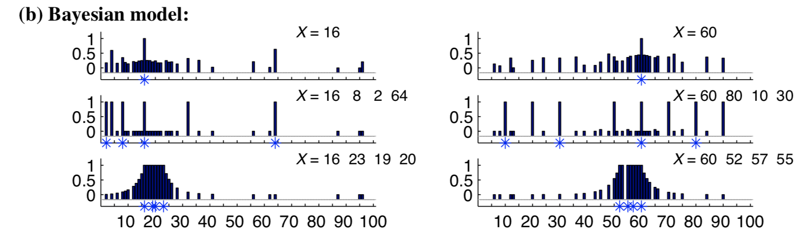
In a task called the number game, participants were presented with sets of numbers and asked how well different numbers completed them. A rule-based generative model accurately captured responses for some stimuli (e.g. for \(16, 8, 2, 64\) or \(60, 80, 10, 30\), participants assigned high fit to powers of two and multiples of ten, respectively). However, it failed to capture others such as the set \(16, 23, 19, 20\). How good is 18, relative to 13, relative to 99?
Exercise 1.1
Using the rule-based model of this task below, examine the posteriors for the following inputs:
[3], [3, 9], [3, 5, 9].
Describe how the posterior probabilities of the rules change based on the observed sets.
Why are they so different despite having the same priors?
Do these results match your intuition?
var maxNumber = 100;

///fold:
var filterByInRange =  function(set) {
  var inRange = function(v) {v <= maxNumber && v >= 0};
  return _.uniq(filter(inRange, set));
}

var genEvens = function() {
  return filter(function(v) {return v % 2 == 0}, _.range(1, maxNumber));
}

var genOdds = function() {
  return filter(function(v) {return (v + 1) % 2 == 0}, _.range(1, maxNumber));
}

var genMultiples = function(base) {
  var multiples = map(function(v) {return base * v}, _.range(maxNumber));
  return filterByInRange(multiples);
}

var genPowers = function(base) {
  var powers = map(function(v) {return Math.pow(base, v)}, _.range(maxNumber));
  return filterByInRange(powers);
}

var inSet = function(val, set) {
  return _.includes(set, val);
}

var getSetFromHypothesis = function(rule) {
  var parts = rule.split('_');
  return (parts[0] == 'multiples' ? genMultiples(_.parseInt(parts[2])) :
          parts[0] == 'powers' ? genPowers(_.parseInt(parts[2])) :
          parts[0] == 'evens' ? genEvens() :
          parts[0] == 'odds' ? genOdds() :
          console.error('unknown rule' + rule))
};
///

// Considers 4 kinds of rules: evens, odds, and multiples and powers of small numbers < 12
var makeRuleHypothesisSpace = function() {
  var multipleRules = map(function(base) {return 'multiples_of_' + base}, _.range(1, 12));
  var powerRules = map(function(base) {return 'powers_of_' + base}, _.range(1, 12));
  return multipleRules.concat(powerRules).concat(['evens', 'odds']);
}

// Takes an unordered array of examples of a concept in the number game
// and a test query (i.e. a new number that the experimenter is asking about)
var learnConcept = function(examples, testQuery) {
 Infer({method: 'enumerate'}, function() {
   var rules = makeRuleHypothesisSpace()
   var hypothesis = uniformDraw(rules)
   var set = getSetFromHypothesis(hypothesis)
   mapData({data: examples}, function(example) {
     // note: this likelihood corresponds to size principle
     observe(Categorical({vs: set}), example)
   })
   return {hypothesis, testQueryResponse : inSet(testQuery, set)}
 });
}

var examples = [3, 9];
var testQuery = 12;
var posterior = learnConcept(examples, testQuery);
viz.marginals(posterior);
Exercise 1.2
Modify the model to include similarity-based hypotheses, represented as numbers generated by sampling from a common interval.
Implement genSetFromInterval to generate all integers in [a, b].
Implement makeIntervalHypothesisSpace to build a list of all possible intervals in [start, end].
For example, makeIntervalHypothesisSpace(1, 4) should produce the following:
["interval_1_2",
 "interval_1_3",
 "interval_1_4",
 "interval_2_3",
 "interval_2_4",
 "interval_3_4"]
Then modify getSetFromHypothesis to account for interval hypotheses.
var maxNumber = 20;

///fold:
var filterByInRange =  function(set) {
  var inRange = function(v) {v <= maxNumber && v >= 0};
  return _.uniq(filter(inRange, set));
}

var genEvens = function() {
  return filter(function(v) {return v % 2 == 0}, _.range(1, maxNumber));
}

var genOdds = function() {
  return filter(function(v) {return (v + 1) % 2 == 0}, _.range(1, maxNumber));
}

var genMultiples = function(base) {
  var multiples = map(function(v) {return base * v}, _.range(maxNumber));
  return filterByInRange(multiples);
}

var genPowers = function(base) {
  var powers = map(function(v) {return Math.pow(base, v)}, _.range(maxNumber));
  return filterByInRange(powers);
}

var inSet = function(val, set) {
  return _.includes(set, val);
}

var makeRuleHypothesisSpace = function() {
  var multipleRules = map(function(base) {return 'multiples_of_' + base}, _.range(1, 12));
  var powerRules = map(function(base) {return 'powers_of_' + base}, _.range(1, 12));
  return multipleRules.concat(powerRules).concat(['evens', 'odds']);
}
///

var genSetFromInterval = function(a, b) {
  // Your code here
}

var makeIntervalHypothesisSpace = function(start, end) {
  // Your code here
}

var getSetFromHypothesis = function(rule) {
  var parts = rule.split('_');
  return (parts[0] == 'multiples' ? genMultiples(_.parseInt(parts[2])) :
          parts[0] == 'powers' ? genPowers(_.parseInt(parts[2])) :
          parts[0] == 'evens' ? genEvens() :
          parts[0] == 'odds' ? genOdds() :
          // Your code here
          console.error('unknown rule' + rule));
};

var learnConcept = function(examples, testQuery) {
 Infer({method: 'enumerate'}, function() {
   var rules = makeRuleHypothesisSpace();
   var intervals = makeIntervalHypothesisSpace(1, maxNumber);
   var hypothesis = flip(0.5) ? uniformDraw(rules) : uniformDraw(intervals);
   var set = getSetFromHypothesis(hypothesis);
   mapData({data: examples}, function(example) {
     observe(Categorical({vs: set}), example)
   })
   return {hypothesis: hypothesis,
           testQueryResponse: inSet(testQuery, set)};
 });
}

var examples = [3, 10];
var testQuery = 12;
var posterior = learnConcept(examples, testQuery);
viz.marginals(posterior);
Exercise 1.3
Now examine the sets [3], [3, 6, 9], and [3, 5, 6, 7, 9].
Sweep across all integers as testQueries to see the ‘hotspots’ of the model predictions.
What do you observe?
d)
Look at some of the data in the large-scale replication of the number game here. Can you think of an additional concept people might be using that we did not include in our model?
e) Challenge! [Extra credit problem]
Can you replicate the results from the paper (reproduced in figure below) by adding in the other hypotheses from the paper?
Exercise 2: Causal induction revisited
In a previous exercise we explored the Causal Power (CP) model of causal learning. However, Griffiths and Tenenbaum [-@Griffiths2005], “Structure and strength in causal induction”, hypothesized that when people do causal induction, they are not estimating a power parameter (as in CP) but instead they are deciding whether there is a causal relation at all – they called this model Causal Support (CS). In other words, they are inferring whether C and E are related, and if so, then C must cause E.
Exercise 2.1
Implement the Causal Support model by modifying the Causal Power model.
var observedData = [{C:true, E:false}];

var causalPost = Infer({method: 'MCMC', samples: 10000, lag:2}, function() {

  // Is there a causal relation between C and E?
  var relation = ...

  // Causal power of C to cause E
  var cp = uniform(0, 1);

  // Background probability of E occurring regardless of C
  var b = uniform(0, 1);

  mapData({data: observedData}, function(datum) {
    // The noisy causal relation to get E given C
    var E = (datum.C && flip(cp)) || flip(b); // modify this line
    condition(E == datum.E);
  })

  return {relation, cp, b};
})

viz.marginals(causalPost);
Exercise 2.2
Inference with the MCMC method will not be very efficient for the above CS model because the MCMC algorithm is using the single-site Metropolis-Hastings procedure, changing only one random choice at a time. (To see why this is a problem, think about what happens when you try to change the choice about whether there is a causal relation.)
To make this more efficient, construct the marginal probability of the effect directly and use it in an observe statement.
Hint: You can do this either by figuring out the probability of the effect mathematically, or by using Infer.
var observedData = [{C:true, E:false}];

var causalPost = Infer({method: 'MCMC', samples: 10000, lag:2}, function() {

  // Is there a causal relation between C and E?
  var relation = ...

  // Causal power of C to cause E
  var cp = uniform(0, 1);

  // Background probability of E occurring regardless of C
  var b = uniform(0, 1);

  var noisyOrMarginal = //..your code here

  mapData({data: observedData}, function(datum) {
    observe(noisyOrMarginal(...), datum.effect)
  })

  return {relation, cp, b};
})

viz.marginals(causalPost);
Exercise 2.3
Fig. 1 of [-@Griffiths2005] (shown below) shows a critical difference in the predictions of CP and CS, specifically when the effect happens just as often with and without the cause. Show by running simulations the difference between CP and CS in these cases.

var generateData = function(numEWithC, numEWithoutC) {
  var eWithC = repeat(numEWithC, function() {return {C: true, E: true}});
  var noEWithC = repeat(8 - numEWithC, function() {return {C: true, E: false}});
  var eWithoutC = repeat(numEWithoutC, function() {return {C: false, E: true}});
  var noEWithoutC = repeat(8 - numEWithoutC, function() {return {C: false, E: false}});
  return _.flatten([eWithC, noEWithC, eWithoutC, noEWithoutC]);
}

var dataParams = [[8, 8], [6, 6], [4, 4], [2, 2], [0, 0], [8, 6],
                  [6, 4], [4, 2], [2, 0], [8, 4], [6, 2], [4, 0],
                  [8, 2], [6, 0], [8, 0]];

var data = map(function(x) { generateData(x[0], x[1]) }, dataParams);

var cpPost = function(observedData) {
  return Infer({method: 'MCMC', burn: 2000, samples: 1000, lag:2}, function() {
    var cp = uniform(0, 1);
    var b = uniform(0, 1);

    var noisyOrMarginal = ...

    mapData({data: observedData}, function(datum) {
      observe(noisyOrMarginal(...), datum.E);
    })

    return cp;
  })
}

var csPost = function(observedData) {
  return Infer({method: 'MCMC', burn: 2000, samples: 1000, lag:2}, function() {
    var relation = ...
    var cp = uniform(0, 1);
    var b = uniform(0, 1);

    var noisyOrMarginal = ...

    mapData({data: observedData}, function(datum) {
      observe(noisyOrMarginal(...), datum.E);
    })

    return cp;
  })
}

var paramNames = map(function(x) {
  var letter = (x + 10).toString(36).toUpperCase();
  var params = dataParams[x];
  return letter + '. (' + params[0] + ', ' + params[1] + ')'
}, _.range(dataParams.length));

var cpValues = map(function(d) { expectation(cpPost(d)) }, data);
var csValues = map(function(d) { expectation(csPost(d)) }, data);

display("Causal power model");
viz.bar(paramNames, cpValues);

display("Causal support model");
viz.bar(paramNames, csValues);
Exercise 2.4
Explain why the Causal Support model shows this effect using Bayesian Occam’s razor.
Hint: Recall that Causal Support selects between two models (one where there is a causal relation and one where there isn’t).
Exercise 3 (Challenge! [Extra credit problem])
Try an informal behavioral experiment with several friends as experimental subjects to see whether the Bayesian approach to curve fitting given on the wiki page corresponds with how people actually find functional patterns in sparse noisy data. Your experiment should consist of showing each of 4-6 people 8-10 data sets (sets of x-y values, illustrated graphically as points on a plane with x and y axes), and asking them to draw a continuous function that interpolates between the data points and extrapolates at least a short distance beyond them (as far as people feel comfortable extrapolating). Explain to people that the data were produced by measuring y as some function of x, with the possibility of noise in the measurements.
The challenge of this exercise comes in choosing the data sets you will show people, interpreting the results and thinking about how to modify or improve a probabilistic program for curve fitting to better explain what people do. Of the 8-10 data sets you use, devise several (“type A”) for which you believe the WebPPL program for polynomial curve fitting will match the functions people draw, at least qualitatively. Come up with several other data sets (“type B”) for which you expect people to draw qualitatively different functions than the WebPPL polynomial fitting program does. Does your experiment bear out your guesses about type A and type B? If yes, why do you think people found different functions to best explain the type B data sets? If not, why did you think they would? There are a number of factors to consider, but two important ones are the noise model you use, and the choice of basis functions: not all functions that people can learn or that describe natural processes in the world can be well described in terms of polynomials; other types of functions may need to be considered.
Can you modify the WebPPL program to fit curves of qualitatively different forms besides polynomials, but of roughly equal complexity in terms of numbers of free parameters? Even if you can’t get inference to work well for these cases, show some samples from the generative model that suggest how the program might capture classes of human-learnable functions other than polynomials.
You should hand in the data sets you used for the informal experiment, discussion of the experimental results, and a modified WebPPL program for fitting qualitatively different forms from polynomials plus samples from running the program forward.